Intro to Databases

Databases are an essential part of modern software development. They allow you to store, retrieve, and manipulate data efficiently. Though a true understanding of database management is beyond the scope of this unit, we will still cover the eseential concepts and commands. We will cover the basics of databases, including how they work, their importance, and the different types of databases available. We will also take a look at SQL, the language used to interact with most databases.

After going through this module, students should be able to understand:

• DBMS and RDBMS

• NoSQL Databases

• Basic database concepts

• What is SQL?

• Basic SQL commands

• Postgres

Database Management Systems

While there are many technical definitions for databases, the best way to think about them is a collection of data that is organized in a way that allows for easy access and manipulation. Usually in order to access your data, you will need to use a database management system (DBMS).

A DBMS is a software application that interacts with the database and allows you to perform operations such as creating, reading, updating, and deleting data. The data can have any structure to it, but most databases are organized in a tabular format, similar to a spreadsheet. These use a specific type of management system called a Relational Database Management System (RDBMS).

RDBMS

An RDBMS is a type of DBMS that is based on the relational model. In a relational model, data is organized into tables, which are made up of rows and columns. This is similar to a spreadsheet you may have worked with such as Google Sheets or Microsoft Excel. It follows a similar structure with clearly defined definitions.

Take a look at the figure below.

There are a few terms that are used similary to any table data that you might already know but just have different names.

Row - A row is a single record in a table. It is also called a tuple or a record

Column - A column is a single field in a table. It is also called an attribute or a field

Table - A table is a collection of rows and columns. It is also called a relation

View - A view is a virtual table that is based on the result of a query. It is also called a virtual table

There are plenty of other terms that are used in database development, but understanding that in the end this is how the data is structured for traditional databases is the most important part.

There are many different types of RDBMS systems, but they all follow the same basic principles. Some of the most popular RDBMS systems including: PostgreSQL, MySQL, SQLite, Microsoft SQL Server, and Oracle Database. You can learn more about each of these systems in the additional resources section at the end of this module.

We will be using PostgreSQL for this unit, but the concepts we will cover will be applicable to any RDBMS system.

Note

Though RDBMS is the most common type of database, there are other types of databases such as NoSQL databases, which are not based on the relational model. These databases to not store data in a tabular format, but rather in a more flexible format such as key-value pairs, documents, or graphs. NoSQL datatabases are beyond the scope of this class, but I encourage you to explore them on your own.

You can learn more about them here - MongoDB - What is NoSQL?

Setup and Installation

You can choose to install PostgreSQL locally on your machine, but you can also leverage something you have already learned to run PostgreSQL in a Docker container.

If you choose to install PostgreSQL locally, you can find the installation instructions here: PostgreSQL Installation

For now though I will be showing how you can run PostgreSQL in a Docker container, though the same commands apply.

1. Pull the PostgreSQL image from Docker Hub

   docker pull postgres:17.4
   

2. Start the PostgreSQL container

   docker run --name postgres -e POSTGRES_PASSWORD=secret -d postgres:17.4
   

3. Connect to the PostgreSQL container

   docker exec -it postgres psql -U postgres
   

The first command pulls the postgres docker image, which should look familar to you.

The second command starts the container and sets the password for the postgres user using the environment variable POSTGRES_PASSWORD. This just sets the super user password for your image if it is required to make any changes.

The third command connects to the PostgreSQL container and opens the PostgreSQL command line interface (CLI) using the psql command. The -U flag specifies the user to connect as, in this case the default super user postgres which is automatically created by Postgres.

Your terminal should now be connect and show a console window like below.

postgres=#

Note

psql is the command line interface for PostgreSQL. It allows you to interact with the database using SQL commands along with their own Postgres commands to view databases, tables, etc.

You can learn more about it here: psql Documentation

SQL

Though data is stored in a relational (tabular) model, true database data is stored in binary format. In order to access this data the RDMBS will offer a query language to access the data.

Different companies and organizations offer different RDBMS systems, from proprietary to open source solutions. However, if they each had their own query language to access the data, then users would have to learn a new language every time they wanted to switch to a new RDBMS.

To solve this problem, a technical standard query language was developed that RDBMS systems could use to access the data called Structured Query Language (SQL). Users now have a standard way to perform different operations on the data, regardless of the RDBMS system they are using.

Note

SQL is a standard language for accessing and manipulating databases, but each RDBMS system may have its own implementation of SQL with some additional features or syntax. This means that while the basic SQL commands are the same across different RDBMS systems, there may be some differences in the way they are used.

You can learn more about the differences between SQL implementations here: SQL Dialects

Basic SQL Commands

Once connected to the PostgreSQL CLI, you can start running SQL commands. You can verify it works by running the following commandand get a printout that looks similar to the one below:

postgres=# SELECT version();

                                                version
---------------------------------------------------------------------------------------------------------------------
PostgreSQL 17.4 (Debian 17.4-1.pgdg120+2) on x86_64-pc-linux-gnu, compiled by gcc (Debian 12.2.0-14) 12.2.0, 64-bit
(1 row)

Attention

Always be sure to end your commands with a semicolon ;. This is how the RDBMS knows you are done with your command. Multiple lines are allowed, but the semicolon is required to execute the command.

CREATE DATABASE

When you first connect to Postgres it will automatically create a database for you called postgres. Since we like to create a database for our own needs, we will specify a new database. You can use the CREATE DATABASE command to create a new database.

Run the following command to create a new database called my_database:

postgres=# CREATE DATABASE my_database;

You can verify that the database was created by running the following command to view the available databases:

postgres=# \l

We then need to connect to the new database in order to create tables and insert data into it.

postgres=# \c my_database

This tells Postgres to connect to the database my_database, and any commands we run from now on will be run in the context of this database.

CREATE TABLE

Now that you are connected to your new database, we need to create a table to store our data. SQL offers the CREATE TABLE command to create a new table. Run the following command to create a new table called users:

CREATE TABLE users (
    id INTEGER PRIMARY KEY GENERATED ALWAYS AS IDENTITY,
    name VARCHAR(255) NOT NULL,
    address  VARCHAR(255),
    age INT NOT NULL
);

Let’s take a more detailed look at the command above.

• Line 1 is using the command CREATE TABLE to create a new table called users.

• Line 2 is defining the first column called id. The data type is INTEGER, which means it can store an integer. The PRIMARY KEY constraint and GENERATED ALWAYS AS IDENTITY attribute are applied to this column as well.

• Line 3 is defining the first column called name. The data type is VARCHAR(255), which means it can store a string of up to 255 characters. The NOT NULL constraint means that this column cannot be empty.

• Line 4 is defining the second column called address. The data type is also VARCHAR(255), but it does not have the NOT NULL constraint, so it can be empty.

• Line 5 is defining the third column called age. The data type is INT, which means it can store an integer. The NOT NULL constraint means that this column cannot be empty.

• Line 6 is closing the command with a closing parenthesis and semicolon.

Line 2 in particular is doing some extra work for us. The PRIMARY KEY constraint means that this column will be the unique identifier for each row in the table. The GENERATED ALWAYS AS IDENTITY means that this column will automatically generate a unique value for each row.

Attention

Each row in your tables should always contain a Primary Key. This unique identifier is valuable and a way to easily access your data and reference it in other tables.

Creating tables follows a similar structure where you define the table name, the columns, and the data types. each comma means that it is a new column that you are defining, until the closing parenthesis and semicolon.

You can verify that the table was created by running the following command to view the available tables:

postgres=# \dt

Note

There are many different data types available in SQL, but each RDBMS system may have its own implementation of these data types. You can learn more about the different data types available in PostgreSQL here:

PostgreSQL Data Types

You can also view the table structure by running the following command:

postgres=# \d users

This will show you the columns, data types, and constraints for the table users.

We have mostly been using psql commands so far, but we will be looking at how similar commands can be run in SQL.

INSERT INTO

Now that we have a table, we can start inserting data into it. With SQL the INSERT INTO command can insert data into a table.

Run the following command to insert a new row into the users table:

INSERT INTO users (name, address, age)
VALUES ('Andrew Solis', '123 Main St', 34);

You should receive an output like the one below:

INSERT 0 1

This means that the command was successful and 1 row was inserted into the table. Let’s try adding a few more rows to the table.

INSERT INTO users (name, address, age)
VALUES ('John Doe', '456 Elm St', 28),
       ('Miguel Hernandez', '789 Oak St', 45),
       ('Rylan Chong', '101 Pine St', 40);

The output now specifies that we have inserted 3 rows

INSERT 0 3

Now we can start to view the data we have inserted into the table.

Exercise 1

1. Create a new table called products with the following columns:

id (integer, primary key, auto-increment)
name (string, not null)
price (decimal, not null)
quantity (integer, not null)
description (string, null)

2. Insert the following data into the products table:

('Laptop', 999.99, 10, 'High-performance laptop')
('Smartphone', 499.99, 20, 'Latest smartphone model')
('Tablet', 299.99, 15, 'Portable tablet device')
('Headphones', 99.99, 30, 'Noise-cancelling headphones')

SELECT

One of the most common commands that you will use in SQL is the SELECT command. This can be used to retrieve data from a table, while also specifying conditions.

Let’s look at a simple example of selecting all the data from the users table:

SELECT * FROM users;

The * means that we want to select all the columns from the table. You should receive an output like the one below:

id  |       name       |   address   | age
----+------------------+-------------+-----
1   | Andrew Solis     | 123 Main St |  34
2   | John Doe         | 456 Elm St  |  28
3   | Miguel Hernandez | 789 Oak St  |  45
4   | Rylan Chong      | 101 Pine St |  40
(4 rows)

But what if we wanted to only select certian columns from the table? We can do this by specifying the columns we want to select:

SELECT name, age
FROM users;

The output should now only show the columns we specified.

Now say we wanted to add some conditions. Maybe specific a minumum or maximum age, or a specific name.

The WHERE clause allows you to add conditions such as matching, less than, greater, and much others.

SELECT <column_name(s)>
FROM <table>
WHERE <condition(s)>;

Say for example we only wanted to select those users that are older than 30:

SELECT *
FROM users
WHERE age > 30;

You should now only receive 3 rows of data, since John Doe is 28 (lucky him).

Or, say we wanted only users who are aged 40.

SELECT *
FROM users
WHERE age = 40;

You can also combine multiple conditions using the AND and OR keywords.

SELECT *
FROM users
WHERE age > 30 AND address = '123 Main St';

There are a variety of operators that can be used in SQL queries to perform comparisons, arithmetic operations, and more. Below is a table of some common PostgreSQL operators:

Operator	Description	Example(s)
=	Equal to	age = 30 name = ‘Andrew’
<> or !=	Not equal to	age != 30
<	Less than	age < 30
>	Greater than	age > 30
<=	Less than or equal to	age <= 30
>=	Greater than or equal to	age >= 30
AND	Logical AND	age > 20 AND age < 40
OR	Logical OR	age < 20 OR age > 40
NOT	Logical NOT	NOT (age = 30)
LIKE	Pattern matching (case-sensitive)	name LIKE ‘A%’
ILIKE	Pattern matching (case-insensitive)	name ILIKE ‘a%’
IN	Matches any value in a list	age IN (25, 30, 35)
BETWEEN	Within a range (inclusive)	age BETWEEN 20 AND 30
IS NULL	Checks if a value is NULL	address IS NULL
IS NOT NULL	Checks if a value is not NULL	address IS NOT NULL

Exercise 2

1. Write a SQL query to select all products with a price greater than 500.

2. Write a SQL query to select all users who live on “Pine St” and are older than 30.

3. Write a SQL query to select all products with a name that starts with “R”.

ALTER TABLE

Once a table has been created by SQL, your data must always follow the structure of the table. However, there may be times when you need to change the structure of the table. Maybe your data changes, or the type of a column needs to be changed.

The ALTER TABLE command allows you to change the structure of a table.

For example, say we wanted to add a new column to the users table called email:

ALTER TABLE users
ADD COLUMN email VARCHAR(255);

Here we specify the command ADD COLUMN to add a new column to the table.

We also specify the data type of the new column, which is VARCHAR(255).

We can now use the SELECT command to see our new table and it’s new column.

Other options that we can use with ALTER TABLE include:

• DROP COLUMN - This will remove a column from the table.

• RENAME COLUMN - This will rename a column in the table.

• ALTER COLUMN - This will change the data type of a column in the table.

You can learn more about these options here: ALTER TABLE

Warning

When adding a column that cannot be NULL, there are some additional steps that need to be taken. You can set the column to have a default value or some computed value.

UPDATE

Now that we have added a column to our table, we now need to update it with information.

The UPDATE follows a similar structure to the INSERT INTO command, but we will be updating existing data and can specify conditions for which data to update.

UPDATE table_name
SET COLUMN1 = value1, COLUMN2 = value2, ...
WHERE condition;

Let’s update the email address for Andrew Solis.

UPDATE users
SET email='asolis.email.com'
WHERE name='Andrew Solis';

Note

If you add special characters to your column names, you will need to use double quotes to access them. Example if "e-mail" is the column then it must be in double quotes, since it has a dash (-) in it.

You can also update multiple columns as well.

UPDATE users
SET address='752 mango blvd', age=35
WHERE name='Andrew Solis';

If we leave the WHERE clause off, it will update all the rows in the table.

UPDATE users
SET email='default.email.com';

Danger

Be careful when using the UPDATE command with or without a WHERE clause. You run the risk of updating data you didn’t mean to update.

DELETE

We’ve been able to alter our table, but say for example we have a user we no longer wish to store their information in our database.

We can use the DELETE command to remove a row from the table.

The DELETE command follows a similar template to what we’ve seen before.

DELETE FROM table_name
WHERE condition;

Say for example we wanted to delete all users with an age of 45.

DELETE FROM users
WHERE age=45;

The same way we used conditions before to specify which rows to delete, we can do the same to specify multiple conditions.

DELETE FROM users
WHERE age=28 AND address='456 Elm St';

What do you think will happen if we don’t include the where clause?

Danger

Be careful when using the DELETE command! You run the risk of deleting data you didn’t mean to delete, including the entire database.

DROP TABLE

Sometimes we need to drop not only a row, but the entire table. Maybe we are no longer using the table and the data has been moved over, or instead of altering the table we have a script and it is easier to just start from scratch.

The DROP TABLE command will remove the entire table and all the data in it.

DROP TABLE table_name;

We can do use this to delete the users table.

DROP TABLE users;

Now try running the SELECT command to see if the table still exists.

Note

You can also use the DROP DATABASE command to remove an entire database and all the tables in it.

DROP DATABASE my_database;

JOINS

Let’s go ahead and create our table again and add in some data.

CREATE TABLE users (
    id INTEGER PRIMARY KEY GENERATED ALWAYS AS IDENTITY,
    name VARCHAR(255) NOT NULL,
    address  VARCHAR(255),
    age INT NOT NULL
);

INSERT INTO users (name, address, age)
VALUES ('Andrew Solis', '123 Main St', 34),
       ('John Doe', '456 Elm St', 28),
       ('Miguel Hernandez', '789 Oak St', 45),
       ('Rylan Chong', '101 Pine St', 40);

SELECT * FROM users;

Our table is starting to look good, but we only have one for now. In reality most databases contain multiple tables. In order to access data from multiple tables, SQL offer JOIN commands.

These can be used to combine rows from two or more tables based on a related column between them.

For example, say each user has a column that is an id for a company they work for that is a separate table.

CREATE TABLE companies (
    id INTEGER PRIMARY KEY GENERATED ALWAYS AS IDENTITY,
    name VARCHAR(255) NOT NULL,
    address  VARCHAR(255),
    phone VARCHAR(255)
);

INSERT INTO companies (name, address, phone)
VALUES ('Google', '123 Google St', '555-555-5555'),
       ('Microsoft', '456 Microsoft St', '555-555-5555'),
       ('Apple', '789 Apple St', '555-555-5555'),
       ('Amazon', '101 Amazon St', '555-555-5555');

ALTER TABLE users
ADD COLUMN company_id INTEGER REFERENCES companies(id);

If we now look at our users table we will see a new column for company_id. This is a foreign key that references the id column in the companies table.

But what exactly is a foreign key?

Foreign Key Tangent

A foreign key is a column or set of columns in one table that refers to a row in another table, usually by the primary key, but they can be referenced in other ways. It establishes a relationship between the two tables and enforces referential integrity. This is particular helpful when you have two tables and need to do a query that involves both tables.

It also solves issues of inserting data into the database where you may require a table to reference another.

Note that we aren’t using the FOREIGN KEY command in the table creation. This is because we are using the REFERENCES command in the column definition. This is a shorthand way of defining a foreign key constraint and Postgres allows this.

If we were to do this through traditional sql it would look like this:

ALTER TABLE users
ADD CONSTRAINT fk_company
FOREIGN KEY (company_id) REFERENCES companies(id);

It would look similar if we created the table with the foreign key constraint already in place.

CREATE TABLE users (
    id INTEGER PRIMARY KEY GENERATED ALWAYS AS IDENTITY,
    name VARCHAR(255) NOT NULL,
    address  VARCHAR(255),
    company_id INTEGER,
    age INT NOT NULL,
    CONSTRAINT fk_company
    FOREIGN KEY (company_id)
    REFERENCES companies(id)
);

End of Tangent

Let’s go ahead and drop all the data in our table and add our data back in, but include a company_id to refernce the companies table.

DELETE FROM users;

INSERT INTO users (name, address, age, company_id)
VALUES ('Andrew Solis', '123 Main St', 34, 1),
       ('John Doe', '456 Elm St', 28, 2),
       ('Miguel Hernandez', '789 Oak St', 45, 3),
       ('Rylan Chong', '101 Pine St', 40, 4);

SELECT * FROM users;

The reason we have been looking at foreign keys is because they are very powerful and useful when performing JOIN commands.

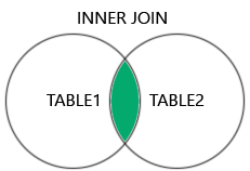
There are multiple types of joins available when querying data from multiple tables. The 4 most common are listed below.

Join Type	Description	Image
INNER JOIN	Returns rows that have matching values in both tables.
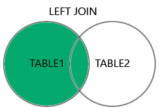
LEFT JOIN	Returns all rows from the left table, and the matched rows from the right table.
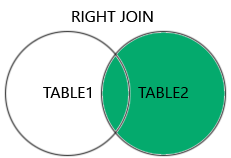
RIGHT JOIN	Returns all rows from the right table, and the matched rows from the left table.
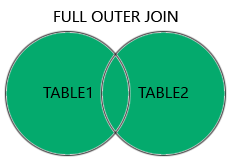
FULL JOIN	Returns all rows when there is a match in either table.

Though you can use different joins, they follow similar query structures.

SELECT <columns>
FROM <table1>
<JOIN Type> <table2>
ON <table1.column = table2.column>;

Let’s modify our data to add companies that have no reference to any existing users, and users that have no reference to any existing companies.

Note

You may have to restart the auto generated primary key for the companies table. This is because the auto incrementing primary key will not reset when you delete the data. You can do this by running the following command:

ALTER SEQUENCE companies_id_seq RESTART WITH 1;

DELETE FROM users;
DELETE FROM companies;

INSERT INTO companies (name, address, phone)
VALUES ('Google', '123 Google St', '555-555-5555'),
       ('Microsoft', '456 Microsoft St', '555-555-5555'),
       ('Apple', '789 Apple St', '555-555-5555'),
       ('Amazon', '101 Amazon St', '555-555-5555'),
       ('Ford', '333 Ford Rd', '555-555-5555'),
       ('Yahoo', '111 Tesla St', '555-555-5555');

INSERT INTO users (name, address, age, company_id)
VALUES ('Andrew Solis', '123 Main St', 34, 1),
       ('John Doe', '456 Elm St', 28, 2),
       ('Miguel Hernandez', '789 Oak St', 45, 3),
       ('Rylan Chong', '101 Pine St', 40, 1),
       ('Ricky Bobby', '111 Pine St', 40, 2),
       ('Kelly Gaither', '222 Pine St', 28, 3),
       ('Donald Tai Loy Ho', '444 Pine St', 28, NULL),
       ('Duke Kahanamoku', '333 Pine St', 45, 1);

Let’s try doing an inner join on our data.

SELECT *
FROM users
INNER JOIN companies
ON users.company_id = companies.id;

Do you notice anything about the data? Any rows from each table that are missing perhaps?

We could also select only those columns we wish to return.

SELECT users.name, users.address, companies.name, companies.address
FROM users
INNER JOIN companies
ON users.company_id = companies.id;

If you look at the output you will see that some column names are similar. We can use the AS keyword to rename the columns in the output.

SELECT users.name AS user_name, users.address AS user_address,
       companies.name AS company_name, companies.address AS company_address
FROM users
INNER JOIN companies
ON users.company_id = companies.id;

Note

Sometimes some RDBMS allow JOIN to be used, which uses the default join type, which traditionally is INNER JOIN.

Let’s now take a look at a LEFT JOIN.

SELECT *
FROM users
LEFT JOIN companies
ON users.company_id = companies.id;

The key difference here is that any rows from the left table (users) will be returned, even if there is no match in the right table (companies). See if you can see in the output a user who is missing a company.

Exercise 3

1. Do a Right Join on the users and companies table and compare the output with the previous joins.

2. Do a Full Join on the users and companies table and compare the output with the previous joins.

Persistent Data

While working with databases in containers is great without having to do a full installation, so far our data only exists in the container. If we stop the container, all the data will be lost.

We learned in Unit 3 how to mount volumes to persist data in containers. Docker also allows you to use Volumes to persist data from containers.

You create a Volume using docker commands and specify the volume you wish to use.

Let’s first exit our container and stop and remove it.

docker stop postgres
docker rm postgres

Now let’s specify the volume we want to create, pgdata.

docker volume create pgdata

By default Postgres stores data in the directory /var/lib/postgresql/data.

The same way how we specified which directories to mount before, we use the same command but instead specify which volume to use.

docker run --name db -e POSTGRES_PASSWORD=secret -v pgdata:/var/lib/postgresql/data -d postgres:17.4

Now any data we create in the container will be persisted in the volume pgdata.

Exercise 4

1. Connect to the docker container as you did before.

   docker exec -it db psql -U postgres
   

2. Copy and Insert the previous data for companies and users into the database.

   CREATE TABLE companies (
       id INTEGER PRIMARY KEY GENERATED ALWAYS AS IDENTITY,
       name VARCHAR(255) NOT NULL,
       address  VARCHAR(255),
       phone VARCHAR(255)
   );
   
   CREATE TABLE users (
       id INTEGER PRIMARY KEY GENERATED ALWAYS AS IDENTITY,
       name VARCHAR(255) NOT NULL,
       address  VARCHAR(255),
       company_id INTEGER,
       age INT NOT NULL,
       CONSTRAINT fk_company
       FOREIGN KEY (company_id)
       REFERENCES companies(id)
   );
   
   INSERT INTO companies (name, address, phone)
   VALUES ('Google', '123 Google St', '555-555-5555'),
          ('Microsoft', '456 Microsoft St', '555-555-5555'),
          ('Apple', '789 Apple St', '555-555-5555'),
          ('Amazon', '101 Amazon St', '555-555-5555'),
          ('Ford', '333 Ford Rd', '555-555-5555'),
          ('Yahoo', '111 Tesla St', '555-555-5555');
   
   INSERT INTO users (name, address, age, company_id)
   VALUES ('Andrew Solis', '123 Main St', 34, 1),
          ('John Doe', '456 Elm St', 28, 2),
          ('Miguel Hernandez', '789 Oak St', 45, 3),
          ('Rylan Chong', '101 Pine St', 40, 1),
          ('Ricky Bobby', '111 Pine St', 40, 2),
          ('Kelly Gaither', '222 Pine St', 28, 3),
          ('Donald Tai Loy Ho', '444 Pine St', 28, NULL),
          ('Duke Kahanamoku', '333 Pine St', 45, 1);
   

3. Stop and remove the container.

4. Start a new container using the same volume.

5. Verify that the data is still there.

Volumes persist even if your computer is restarted, but they can be removed. They follow a similar command to what we’ve seen before.

docker volume rm pgdata

You can also run the prune command which will remove all unused volumes.

docker volume prune

These commands will only work though if the volume is not connected to any other container.

You can force the volume to be removed while also stopping any containers connected to it using the following command:

docker volume rm -f pgdata

Common psql Commands

Command	Description
\l	List all databases
\c <db_name>	Connect to a specific database
\d	List all tables, views, and sequences in the database
\dt	List all tables in the current database
\d <table_name>	Describe the structure of a specific table
\du	List all roles (users)
\q	Quit the psql command-line interface
\i <file_name>	Execute SQL commands from a file
\x	Toggle expanded table output format
\password	Change the password for the current user

Additional Resources

Materials in this module were based in part on the following resources:

W3 Schools PostgreSQL Tutorial

W3 Schools SQL Tutorial

Persistent Container Data

SQL

SQL Cheat Sheet | SQL Reference

RDBMS

PostgreSQL | SQLite | MySQL | Microsoft SQL Server | Oracle Database

NoSQL DBMS

MongoDB | Cassandra | Redis